Generally, the use of simulation technologies within product development is restricted to two key areas. The first, and perhaps the oldest, is to discover why a particular fault has occurred. Failure analysis is still prevalent and while highly useful, it’s really a case of bolting the stable door once the horse is long gone.
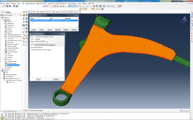
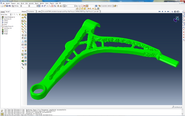
Optimisation Task created and appropriate region of the model is selected. The orange elements are where the optimisation will take place, leaving mounting components as found
The other scenario is often along the lines of ‘I’ve designed this, will it break?’ Again, this is a perfectly valid approach; develop a product using all of the tools available then sanity check the resultant form to ensure nothing has been missed.
Much of the two workflows are driven by previous experience, group knowledge and best practices – as you might expect. But the simulation tools are essentially doublechecking your knowledge, rather than expanding or enhancing it. Surely there’s something in today’s technologicallyled world that allows the design and engineering user to work a little smarter?
The answer is “yes” – and it’s called optimisation. By combining the wealth of simulation techniques available it’s now possible to use your design parameters and functional requirements to drive the design of a part, or even group of parts. By using a series of experiments, it’s possible to explore the range of design scenarios and find the optimum form that satisfies all the requirements.
There are many methods available to do this, but one of the most intriguing has always been topology optimisation. You begin with a basic rough model of a part. Consider this a rough billet that possesses the basic required form, in terms of both dimensions and geometric features. The optimisation engine then removes material from that form until it achieves the goals that have been set.
The key difference between parametric and topology optimisation is that the former is constrained by the nature and number of parameters selected as variables whereas the latter is a much more global approach that usually results in greater design improvements.
However, topology optimisation does allow design constraints for practical considerations such as manufacturability. With parametric optimisation you define what you can vary and everything else is fixed; with topology optimisation everything is variable except what you decide to constrain.
The Abaqus Topology Optimisation Module (ATOM) differs from these types of tools in two ways.
The first is that it handles both linear and non-linear analyses. That means that components undergoing either large deformation, performing outside of their elastic limit or that are involved in contact, can be optimised. The second is that the system supports both topology optimisation and shape optimisation methods, which we’ll get onto shortly.
But let’s first look at the topology optimisation tools and how to go about setting up a study.
Optimising by topology
The starting point is a sound baseline Abaqus simulation study. This should feature the set-up of the part being looked at to optimise and converge to a satisfactory solution. This is then used as the basis for the iterative optimisation process.
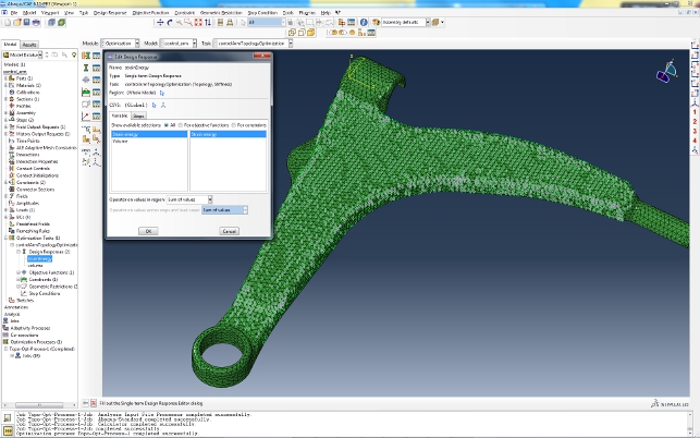
The next stage is to use the familiar Abaqus/CAE environment tools to set-up the design responses for the study. These are the factors that define how the component performs and the metric that will be used as part of the optimisation process for both input and output. They can include centre of gravity, displacements, strain energies, volumes, forces, velocities etc.
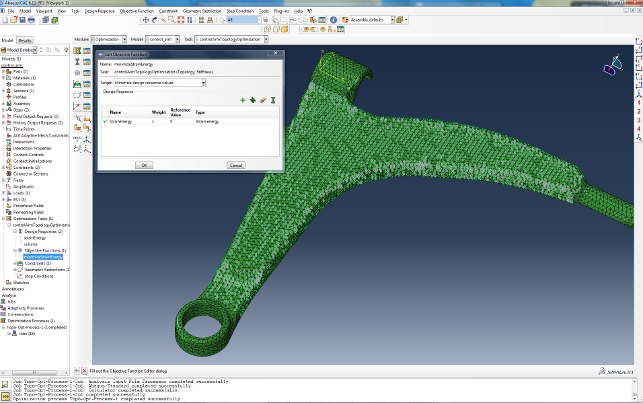
The next step is to define the objective functions for those design responses. Here things become interesting because multiple objectives can be added to give each a weighting in terms of priority and influence over the process.
For example, the user might be looking to reduce the weight of a component, but also need to ensure that the stiffness and centre of gravity remain within specific ranges.
This should provide the basic set-up of factors that are both resultant from the process and input into the optimisation process.
After defining the objectives of the optimisation, the user has the option of providing constraints on the optimisation simulation. For example, the volume of the optimised model can be constrained to be 50% of the original volume. The user selects one of the design responses defined previously and enters the appropriate constraint value.
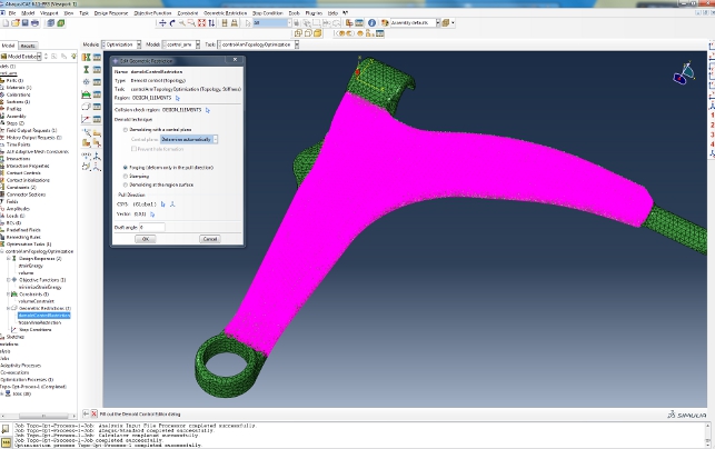
The next stage is to define geometric restrictions within which the optimisation takes place. These can range from basics such as selecting areas of the component that can’t be modified, through to specific member size and into things like symmetry.
Alongside these, there is also a host of manufacturing – or processing – related restrictions such as the requirement for de-moulding, forging or stamping. These constraints are required as, for example with a forged component, the optimisation will add or remove material only in the pull direction of the operation.
The last pre-processing step is to submit the job for solving. The system asks for the maximum number of iterations that can be run. This is submitted using the Job Manager, as with any Abaqus analysis.
Method, results and workflow
Within these tools, the objective function is to minimise the total strain energy calculated from all the elements. The constraints force the optimisation to reduce the volume.
During the optimisation, the density and the stiffness of the elements are reduced so that the elements are, in effect, ‘removed’ from the analysis. However, the elements are still present, and they could play a later role in the analysis if their density and stiffness increase as the optimisation continues.
For post processing the user loads up the data deck to work through the various iterations and explore the results to show the final optimum design.
For topology optimisation, the system uses iso-surface display to show each iteration by hiding the elements that’s zero-ed out.
The results are a tessellated mesh. In terms of an onward path for the workflow, the concept is to arrive at the optimised result and then export it as an STL.
This can then be imported into the user’s workhorse 3D design tool as a reference and proper geometry modelled up, presumably with subsequent simulations to validate the form and function.
Shape optimisation
The Shape optimisation tools differ in that they are aimed at much more micro level work. These tools tweak the position of the nodes on which the meshes are built to achieve the required outcome. As a result, the user is only looking at very small scale movements.
The set-up processes are very similar but with the shape optimisation tools, the user is looking to refine a specific area of the form, whether that’s to relieve stress concentration, contact stresses or plastic strains.
Again, the results can be inspected, though the iso-surface tools won’t be needed. The data can then be used as reference for further rework in the design system.
It’s also worth noting that using the combination of the two techniques means that the optimised design can be achieved in the first few passes using topology-related tools with the shape optimisation tools used to refine and smooth it out.
Conclusion
The tools we’ve covered are all built into Abaqus/CAE (as a cost option of course) and are available on both the Linux and Windows versions of the system.
Optimisation is a calculation-heavy process so any form of parallel processing you can throw at it, the better. And let’s be honest, Abaqus is not the sort of system that is run on a standalone workstation.
Typical Abaqus customers are going to be working in a multi-core or cluster-based environment, so there’s no real need for anything different. You can pick up these tools and run with them.
www.simulia.com
| Product | ATOM |
|---|---|
| Company name | Simulia |
| Price | on application |