In the previous article we made a 3D model of a U-shaped load cell and observed that, while the in-plane stresses were large, the through-thickness stresses were small.
Thus we used the “plane stress” approximation (zero stress through-thickness) in order to construct an equivalent 2D model. We observed that the governing stresses in the 2D model weren’t overly different to those of the full 3D model. Now we are going to examine how the 3D model was constrained…
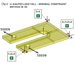
{fig.1} shows the complete 3D solid model of the load-cell with the two bores loaded by 5000N apiece. Note we have opted not to use symmetry.
The applied load should be applied by way of a pressure distribution (a constant pressure over 180-degrees will suffice) and not by some sort of rigid element or constraint pattern. In practice the load-cell plate will experience a contact pressure distribution due to the pin fitted through the bore – for realistic loading we must replicate that.
You should be able to pressurise both bores such that the net thrust applied to each is 5000N vertically. Done correctly you will render the plate in force and moment equilibrium – no net thrust and no net moment results on the plate.
The problem now is how we constrain such a model: balanced loads are applied such that they cause plenty of stress in our component but presently the model is free to translate in the X, Y and Z directions and is free to rotate about the X, Y and Z axes. You could cover one side of the model in weak springs but the most conservative thing to do is to apply a so-called “3-2-1 minimal constraint”.
{fig.1} shows that a corner node is constrained in all three translational freedoms; a second is constrained in two translational freedoms and a third node in one translational freedom. Thus the complete model has six global degrees of freedom (three translations and three rotations) and we have constrained six translations at three wide-spaced non co-linear nodes in order to nullify these global freedoms.
To explain further: the constraint pattern is started by selecting one node (node “A” at the corner of the model) and constraining this in the X, Y and Z translational directions. In a solid model such as this nodes only have translational freedoms so we are not breaking any rules.
Moving away from point “A” we can move to another corner of the model (node “B”) and here constrain the two freedoms normal to the line we just “walked” along.
Finally we move away from the aforementioned line (between nodes “A” and “B”) and identify a third node (designated “C”) and constrain the translational freedom normal to the plane containing nodes “A”, “B” and “C”. The method seems over-complicated at first but with a little practice it is very straightforward and easy to apply.
The “3-2-1” constraint pattern allows the plate to deform in any manner – the constraints applied do not stiffen the component in any way and hence provide conservative stresses. The applied constraints are just sufficient for the analysis to complete and no more.
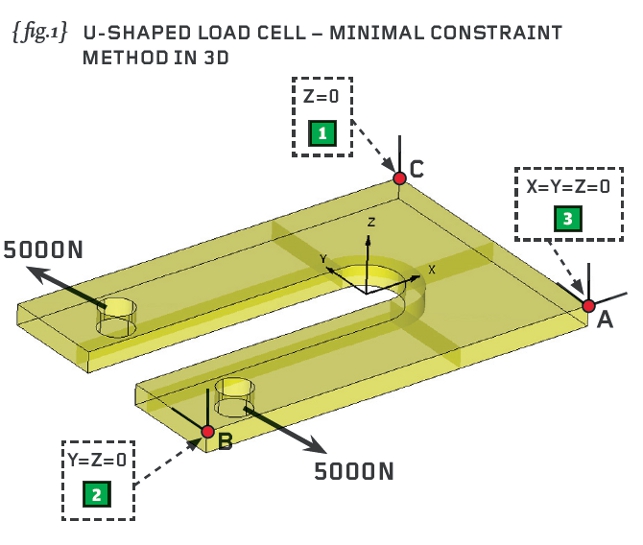
We will now progress to a more complicated Finite Element simulation. {fig.2} shows a detail view of my Scott Genius MC30 mountain bike.
The bike has telescopic forks at the front and a system of linkages at the back in order to provide rear suspension. {fig.2} shows a typical layout of two linkages in parallel such that the movement of the back wheel (with respect to the frame) can be controlled through an air spring and shock absorber. Linkages such as this are commonplace in a wide range of industries.
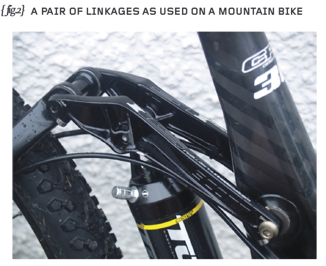
{fig.3} shows a simplified linkage with a main bore, designated “O” and two smaller bores designated “A” and “B”. The principal dimensions of the linkage are added to {fig.3} (in inches).
The applied loading is defined as 1950 pounds-force at bore “A” (normal to the line “O”-“A”) and 1100 pounds-force vertically applied at bore “B”. Given that smooth pivot pins are to be installed in all three bores, is the applied loading sensible? If it is a feasible form of loading then calculate the reactions that the large pin must apply to the linkage.
We will continue with the analysis of the linkage next time when, hopefully, you will have completed your homework! 
Part fourteen of an engineering masterclass: “art” of applying realistic constraints
Default