In order that this instalment can be understood without the figures and text from the previous article, let us summarise where we are to date.
{ fig.1} shows an imaginary switch housing comprising two polyethylene sleeves, one inside the other. The inner sleeve (high density polyethylene, E=440MPa) is loaded 450N downward while the outer sleeve (low density polyethylene, E=180MPa) is constrained from axial movement. The two sleeves are joined together by a steel collar and we assume that the collar is very stiff compared to the two plastic components.
We designate the inner sleeve as element number [1], the outer sleeve as element number [2] and we use three nodes to connect them together. [N.B. It is interesting to observe that one element lies on top of the other and we will return to that issue at a later date]. Each of the nodes has a single “degree-of-freedom” – they can only move in the vertical direction.
Last time we concluded by calculating the basic “spring stiffness” for both parts and we showed that this was equal to EA/L (product of Young’s Modulus and area divided by the effective length).
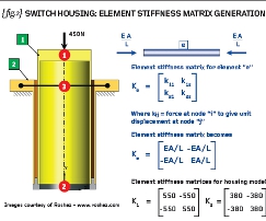
{ fig.2} shows any “general” element and we will refer to that as element “e”. The Finite Element Method requires that an “element stiffness” matrix be defined. In this simple truss model the element stiffness matrix comprises the terms k11/k12/k21/k22 where the general coefficient kij is the force at node “i” to give unit displacement at node “j”. We can see therefore that the leading diagonal terms are the spring stiffness values (EA/L) while the trailing diagonal terms are the same but negative.
We don’t need to get too hung up in the mathematics BUT it is important to realise that each column in the element stiffness matrix is a set of forces in EQUILIBRIUM. The element stiffness matrices for elements [1] and element [2] can be populated therefore with the spring stiffness values of 550N/mm and 380N/mm respectively. Refer to { fig.2}.
At this stage we have the stiffness matrices for the two individual truss elements – these stiffness matrices contain the loads to give unit displacement at one node while all other displacements are zero.
In order to make progress we need to think about the general equation of motion so it may be a good time to go and get a cup of tea before reading on…
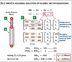
{ fig.3} (top) shows the general equation of motion. Don’t be too put out – this equation just states that some inertia loads (mass x acceleration) plus some damping loads (damping factor x velocity) plus some stiffness loads (stiffness x displacement) within the structure are equal to a set of external loads. There is an implied solution to this set of equations if we neglect acceleration and velocity effects and we can solve the reduced set of equations which are [K]{x}={F}.
The reduced equation of motion [K]{x}={F} now needs to be expressed as a matrix equation. The matrix expression will have M number of equations where M is the product of the number of nodes in our model (three in this case) and the number of degrees-of-freedom at each node (one in our case). The matrix equation requires a square matrix definition of the global stiffness matrix (MxM), a vector containing all the unknown displacements (Mx1) and a vector of external loads (Mx1).
The global stiffness matrix is derived from an assembly of all the element stiffness matrices. Compatibility (continuity) is used to affect this assembly – where displacements are equal then we add the corresponding stiffness terms. In the example shown { fig.3} we note that the displacement at node 2 according to element [1] is exactly the same as the displacement at node 2 according to element number [2]. Thus we add the corresponding stiffness terms such that the global stiffness term in the second row and second column (K22) is the addition of 550N/mm and 380N/mm (making 930N/mm).
In order to arrive at a unique solution we must apply constraints to our set of equations and here we impose the displacement at node number 3 to be zero. Note that the corresponding term in the external loads vector is set to R3 indicating that this is a reaction force to be calculated at a later date. That leaves us with two unknown displacements and two equations so we can happily solve for u1= -2.002mm and u2= -1.184mm. The displacements therefore are the primary unknowns and we have found the cornerstone of our Finite Element (implicit) solution.
Next time we will calculate the reactions and the element stresses and strains. 
Part eleven of an engineering masterclass: Basic Principles of FEA – Part 2


